An Example Vignette

library(bis557)
library(palmerpenguins)
library(DT)

data(penguins)

datatable(penguins)

Above is the penguins data set form the {palmerpenguins} package.

Selecting variables and creating a table

library(dplyr)
#> 
#> Attaching package: 'dplyr'
#> The following objects are masked from 'package:stats':
#> 
#>     filter, lag
#> The following objects are masked from 'package:base':
#> 
#>     intersect, setdiff, setequal, union
library(ggplot2)

# The "base" way.
table(penguins$species, penguins$island)
#>            
#>             Biscoe Dream Torgersen
#>   Adelie        44    56        52
#>   Chinstrap      0    68         0
#>   Gentoo       124     0         0

# The "tidy" way.
penguins %>%
  select(species, island) %>%
  table()
#>            island
#> species     Biscoe Dream Torgersen
#>   Adelie        44    56        52
#>   Chinstrap      0    68         0
#>   Gentoo       124     0         0

Filtering rows

base

table(penguins[penguins$species == "Adelie", "sex"])
#> 
#> female   male 
#>     73     73

tidy

penguins %>%
  filter(species == "Adelie") %>%
  select(sex) %>%
  table()
#> .
#> female   male 
#>     73     73

Building a model

Let’s fit the model:

\[ \text{bill_length_mm} \sim \text{species} \, \beta_1 + \text{island} \, \beta_2 + \text{sex} \, \beta_3 + \beta_0 \]

To fit the model we’ll run the following code:

fit <- lm(bill_length_mm ~ species + island + sex, data = penguins)
summary(fit)
#> 
#> Call:
#> lm(formula = bill_length_mm ~ species + island + sex, data = penguins)
#> 
#> Residuals:
#>     Min      1Q  Median      3Q     Max 
#> -6.3264 -1.3351  0.0149  1.2273 11.0149 
#> 
#> Coefficients:
#>                  Estimate Std. Error t value Pr(>|t|)    
#> (Intercept)       37.1263     0.3729  99.550   <2e-16 ***
#> speciesChinstrap  10.3474     0.4216  24.541   <2e-16 ***
#> speciesGentoo      8.5465     0.4102  20.834   <2e-16 ***
#> islandDream       -0.4886     0.4702  -1.039    0.300    
#> islandTorgersen    0.1026     0.4877   0.210    0.833    
#> sexmale            3.6975     0.2549  14.508   <2e-16 ***
#> ---
#> Signif. codes:  0 '***' 0.001 '**' 0.01 '*' 0.05 '.' 0.1 ' ' 1
#> 
#> Residual standard error: 2.325 on 327 degrees of freedom
#>   (11 observations deleted due to missingness)
#> Multiple R-squared:  0.822,  Adjusted R-squared:  0.8193 
#> F-statistic:   302 on 5 and 327 DF,  p-value: < 2.2e-16

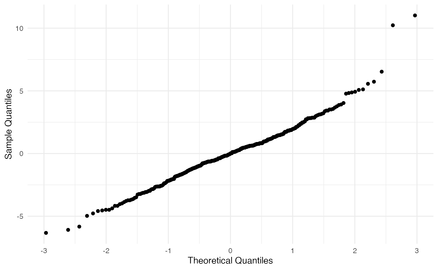
Plot the residuals

library(ggplot2)
# base
qs <- qqnorm(fit$residuals, plot.it = FALSE)
qsd <- as.data.frame(qs)
ggplot(qsd, aes(x = x, y = y)) + 
  geom_point() +
  ylab("Sample Quantiles") +
  xlab("Theoretical Quantiles") +
  theme_minimal()

# tidy
qqnorm(fit$residuals, plot.it = FALSE) %>%
  as_tibble() %>%
  ggplot(aes(x = x, y = y)) + 
    geom_point() +
    ylab("Sample Quantiles") +
    xlab("Theoretical Quantiles") +
    theme_minimal()